Static species distribution models in the marine realm: the case of baleen whales in the Southern Ocean

Aim: Information on the spatiotemporal distribution of marine species is essential for developing proactive management strategies. However, sufficient information is seldom available at large spatial scales, particularly in polar areas. The Southern Ocean (SO) represents a critical habitat for various species, particularly migratory baleen whales. Still, the SO’s remoteness and sea ice coverage disallow obtaining sufficient information on baleen whale distribution and niche preference. Here, we used presence-only species distribution models to predict the circumantarctic habitat suitability of baleen whales and identify important predictors affecting their distribution.
Location: The Southern Ocean (SO)
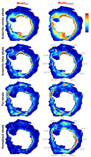
Methods: We used Maxent to model habitat suitability for Antarctic minke, Antarctic blue, fin, and humpback whales. Our models employ extensive circumantarctic data and carefully prepared predictors describing the SO’s environment and two spatial sampling bias correction options. Species-specific spatial-block cross-validation was used to optimise model complexity and for spatially-independent model evaluation.
Results: Model performance was high on cross-validation, with generally little predicted uncertainty. The most important predictors were derived from sea ice, particularly seasonal mean and variability of sea ice concentration and distance to the sea ice edge.
Main conclusions: Our models support the usefulness of presence-only models as a cost-effective tool in the marine realm, particularly for studying the migratory whales’ distribution. However, we found discrepancies between our results and (within) results of similar studies, mainly due to using different species data quality and quantity, different study area extent, and methodological reasons. We further highlight the limitations of implementing static distribution models in the highly dynamic marine realm. Dynamic models, which relate species information to environmental conditions contemporaneous to species occurrences, can predict near-real-time habitat suitability, necessary for dynamic management. Nevertheless, obtaining sufficient species and environmental predictors at high spatiotemporal resolution, necessary for dynamic models, can be challenging from polar regions.