Fin whale (Balaenoptera physalus) distribution modeling on their Nordic and Barents Seas feeding grounds
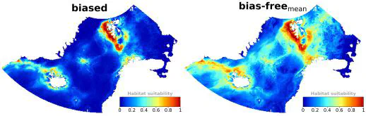
Understanding cetacean distribution is essential for conservation planning and decision-making, particularly in regions subject to rapid environmental changes. Nevertheless, information on their spatiotemporal distribution is commonly limited, especially from remote areas. Species distribution models (SDMs) are powerful tools, relating species occurrences to environmental variables to predict the species’ potential distribution. This study aims at using presence-only SDMs (MaxEnt) to identify suitable habitats for fin whales (Balaenoptera physalus) on their Nordic and Barents Seas feeding grounds. We used spatial-block cross-validation to tune MaxEnt parameters and evaluate model performance using spatially independent testing data. We considered spatial sampling bias correction using four methods. Important environmental variables were distance to shore and sea ice edge, variability of sea surface temperature and sea surface salinity, and depth. Suitable fin whale habitats were predicted along the west coast of Svalbard, between Svalbard and the eastern Norwegian Sea, coastal areas off Iceland and southern East Greenland, and along the Knipovich Ridge to Jan Mayen. Results support that presence-only SDMs are effective tools to predict cetacean habitat suitability, particularly in remote areas like the Arctic Ocean. SDMs constitute a cost-effective method for targeting future surveys and identifying top priority sites for conservation measures.