Improved species-occurrence predictions in data-poor regions: using large-scale data and bias correction with down-weighted Poisson regression and Maxent
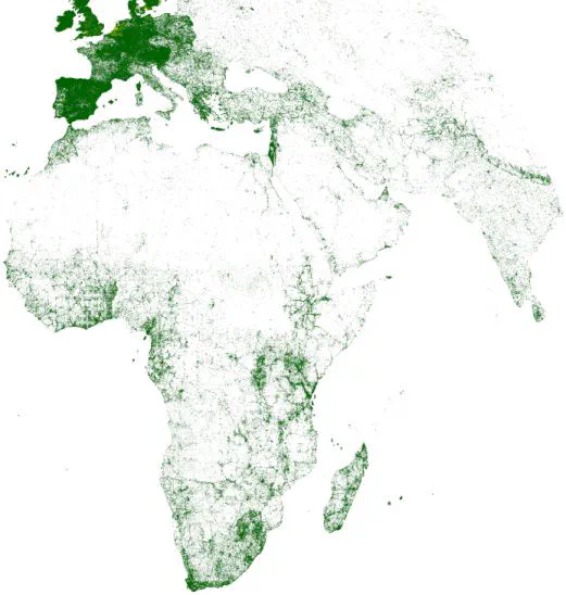 GBIF
GBIF
Species distribution modelling (SDM) has become an essential method in ecology and conservation. In the absence of survey data, the majority of SDMs are calibrated with opportunistic presence-only data, incurring substantial sampling bias. We address the challenge of correcting for sampling bias in the data-sparse situations of developing countries. We modelled the relative intensity of bat records in their entire range using three modelling algorithms under the point-process modelling framework (GLMs with subset selection, GLMs fitted with an elastic net penalty, and Maxent). To correct for sampling bias, we applied model-based bias correction by incorporating spatial information on site accessibility or sampling efforts. We evaluated the effect of bias correction on the models’ predictive performance (AUC and TSS), calculated on spatial-block cross-validation and a holdout data set. When evaluated with independent, but also sampling-biased test data, correction for sampling bias led to improved predictions. The predictive performance of the three modelling algorithms was very similar. Elastic-net models have intermediate performance, with slight advantage for GLMs on cross-validation and Maxent on hold-out evaluation. Model-based bias correction is very useful in data-sparse situations, where detailed data are not available to apply other bias correction methods. However, bias correction success depends on how well the selected bias variables describe the sources of bias. In this study, accessibility covariates described bias in our data better than effort covariates, and their use led to larger changes in predictive performance. Objectively evaluating bias correction requires bias-free presence-absence test data, and without them the real improvement for describing a species’ environmental niche cannot be assessed.